Scientist and engineers use drawings of arrows to denote position and motion. They are called vectors and using them makes many motion-related problems much easier.
Doodling is a crucial and empowering tool used by artists, scientists, and engineers. Many great inventions, many ideas that have changed the world, were born out of a lively conversation and scribble on a napkin. The process of rendering our ideas in drawings allows us to clarify and better understand our own thoughts and leads us to more clearly communicate our ideas to others.
One of the most important elements of many scientific doodles is the arrow. We use arrows to denote directions, positions, orientations, flows, motions, and a myriad other properties and phenomena. We use longer arrows to denote faster movement or larger displacement or more intense flows. And we orient the arrows differently, to denote different directions and positions. By the end of the lesson, you will use arrows in just this way to describe concepts like velocity and acceleration. But first, let’s start with an informal doodle to get the hang of it.
Using Vectors
The specific arrows we introduced above are called vectors by scientists and mathematicians. Knowing the special name for important concepts helps scientists communicate more effectively and makes it easier to find out more about topic. When searching in the library (or on the internet) for more information, it certainly does make it easier to know to look for information on vectors instead of “the type of arrows scientists use in their doodles”. Now that we know the name for this concept, let’s dive deeper.
Position and Displacement
The most immediate application of our arrow doodles (vectors), is to denote a position in space and how that position changes. We would need a starting point with respect to which we will denote all other positions. Imagine you are at that starting point. Then you take a few more steps in an arbitrary direction and you are at a new location. You can draw a vector between the starting position and the initial position. This vector then represents your displacement. We can endow the starting point with the special property of being the center of our map. Frequently this center is called the origin of our map. Vectors starting at that origin can be thought of representing not only displacement, but also a current position.
However, what if you want to represent a more complicated journey? Maybe after stopping at Location 1, you then move to Location 2. This second displacement will be denoted by a second vector. In the journey represented in the image below, one more step is taken to reach the final destination (and a third vector represents that stage).
An important concept comes up when we try to describe the final destination of the journey. The final position is the result of all preceding displacements. It almost feels natural to call the final position the sum of all preceding displacements. But notice this is a different type of addition that the one we have seen before with numbers. It is not only the size that matters here, but also the orientation. We have a special name for this type of operation. We call it vector addition.
By framing vectors as representing motion, the idea of vector addition becomes easier to understand. VectorWe denote variables representing vectors with a cute little arrow above the letter. \(\vec{A}\) represents the first displacement. Then vector \(\vec{B}\) and \(\vec{C}\) represent the second and third steps of our journey, each in a slightly different direction.
Then we can write \[\vec{D} = \vec{A}+\vec{B}+\vec{C}\] and from the drawing we can see that \(\vec{D}\), the vector representing the final position, is the one connecting the starting point and the end destination. It is also the vector obtained by following one after the other each of the vectors representing the sequence of displacements. In other words, to add to vectors together, we simply put the start of the second vector where the first vector ends. Then the new vector, joining the start of the first vector and the end of the second vector, represents the sum, i.e. the total displacement.
Velocity Vectors
Motion, however, is not always described by a few discrete steps. Usually, motion is a smooth process in which the position of a point slowly and smoothly changes, very much unlike the abrupt discrete steps seen above.
Vectors become even more useful here. They permit us to neatly introduce the notion of instantaneous velocity (“instantaneous” is just a fancy word for “current”). This would be a vector whose orientation points along the current direction of motion. This vector is longer if the position is changing faster (a longer vector represents a higher speed), or shorter if the position is changing slowly.
Below you are provided with an interactive visualization of the notion of a velocity vector. You can pick the velocity by dragging the black dot with the cursor of your mouse. In the left circle, the velocity vector will be visualized. This would be the velocity with which the position (in blue) depicted in the right rectangle would be modified. Notice that when the orange velocity vector is small, then the blue position vector changes very slowly. Notice as well that the direction in which the position vector changes is governed by the direction of the velocity vector.
Acceleration Vectors
In many circumstances it is not easy to keep a steady velocity (and hence a steadily changing position). To study such cases, we need to define a new vector, the acceleration vector, which describes how the velocity vector changes. In the same way in which the velocity vector’s direction shows the direction in which the position changes, the acceleration vector’s direction shows how the current velocity will change. And the bigger the acceleration vector is, the more rapidly the velocity vector changes. In the visualization below you can see how changing the acceleration vector (by dragging the black circle) will induce a change in the velocity vector, which in turn will change the velocity.
There are a couple of interesting cases to consider. Try to reproduce the following in the visualization:
- When the acceleration vector points in the same direction as the velocity vector, then the velocity will grow.
- When the acceleration vector is pointing in the direction opposite to the velocity vector, then the velocity will become lower and lower, until eventually the position stops changing. If we continue after that point, the velocity will change directions and start growing bigger and bigger.
- When the acceleration is perpendicular to the velocity, then the velocity will have its orientation change, causing a turn. Try, for instance, to see whether you can control the acceleration such that the position traces out circles.
Vector Magnitude and Components (or Coordinates)
Now that you have become comfortable with drawing vectors, we will begin to describe their properties using numbers. This is particularly useful when we want to use computers to draw vectors, or when we want to learn a vector that was measured by a sensor. For instance, the motion sensors on the SpinWheel can measure the acceleration vector describing the motion of the device. However, to interpret that measurement we need to understand how a vector can be represented as a sequence of numbers.
As we have seen, one important property of vectors is their length. Mathematicians usually call it magnitude or norm. To also describe the orientation of a given vector, we will need something more. We have already mentioned that an origin or a center from which vectors radiate would be convenient. That gives us a reference starting point, but it does not yet give us a reference orientation with respect to which we can measure the orientation of our vector.
One way to achieve this orientation requirement is to draw a grid over which the vectors will be drawn. For a real-world example, consider the tile floor in a cafeteria.
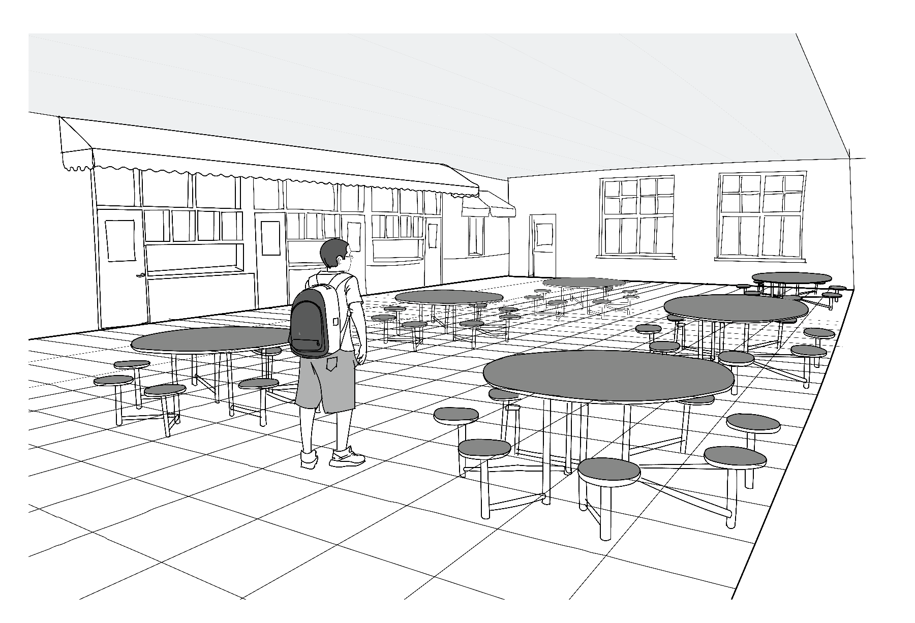
You can pick a tile at the center of the room to be your origin. But the grid provides you with something more: the two sides of the tile give you two axes along which displacement can be measured. To each displacement vector you can assign a description in words: “I move \(X\) tiles to the right and \(Y\) tiles forward”. The numbers \(X\) and \(Y\) is what we call the coordinates (or components) of the vector. It is customary for drawings to depict \(X\) horizontally and \(Y\) vertically.
This custom is kept in the visualization below, where a tile grid is drawn, together with a position vector on top of it. You can use the sliders to modify the coordinates (i.e. the number of tiles taken to the right or forward, where negative numbers are interpreted as stepping to the left or backwards).
A third direction can be added if we want to describe a position in three dimensions. For instance, in the example of a cafeteria with a tile floor, the third component of the vector would be the height above the floor (usually denoted as \(Z\)). Similar grids can be constructed for velocity vectors and acceleration vectors (the grids are called coordinate systems).
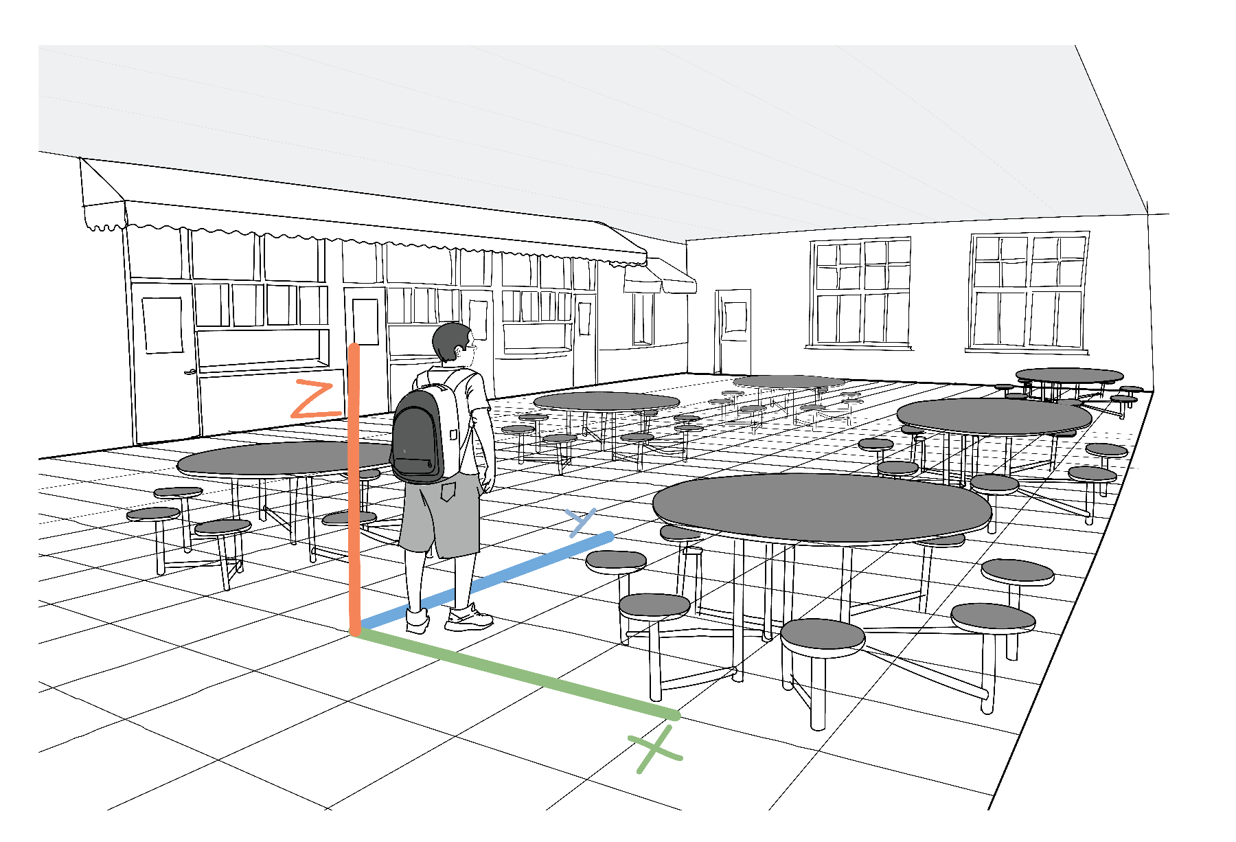
In fact, our SpinWheel device has its own grid in which it measures acceleration. The way this measurement is provided, is as three variables, \(a_x\), \(a_y\), and \(a_z\), which represent the components of the acceleration along the \(X\), \(Y\), and \(Z\) directions. Now that you have a rough understanding of what these number represent, we will use them in various creative endeavors, where a small piece of code will be able to react to motion in a colorful way. For instance, consider how we use acceleration measurements in the Step Counter Adventure, or their more artistic use in the Dancing with Color adventure.
