Rotation and Moving in Circles

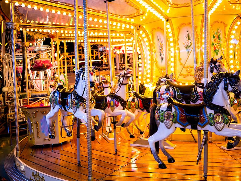
Imagine you are getting on a merry-go-round. Out of the many colorful options, you choose to ride your favorite horse on the outer row. The operator starts the ride, and you begin traveling around under flashing lights and bright mirrors. Now what would have been physically different about this ride had you chosen a different horse? You’ll be able to answer this by the end of the lesson!

This lesson will focus on understanding the many things around us that rotate. Whether it’s a frisbee, a tire wheel, a dancer, or even yourself on an amusement park ride, rotation is all around us. When objects move in straight lines, we call this linear motion. In our Vectors and Motion lesson, we discussed how to describe linear motion. How about rotational motion? What tools do we have to explain this motion?

Angular Displacement

When dealing with circular motion or rotation (for instance, for a ball on a string or a horse on a merry-go-round), it is useful to describe position using an angle (denoted as \(\theta\), pronounced ‘theta’). The change between the original angle of the ball and its final angle is typically specified as the change in \(\theta\) (or \(\Delta \theta\)) and is known as angular displacement. Displacement is a useful term to describe an object’s change in position and can be defined as an angle (angular displacement) or distance (linear displacement). This concept is easier to understand through diagrams. In the image below you can see how linear displacement and angular displacement are related to each other.

Angular Velocity

To describe the motion of a ball as it is spun around on a string or how fast a dancer spins, we use something called angular velocity. Usually when we think of velocity, we are thinking of linear velocityThis type of velocity is sometimes also called translational velocity. defined as the change in position (displacement) during a specified interval of time. Angular velocity is very similar, but it is instead defined as the change in angle over time. While angular velocity and linear velocity are related they are not the same. For instance, take our ball, if we change the length of the string, we can keep our angular velocity the same, but the linear velocity will be different. You can experiment below with how changing the length of the string changes the angular and linear velocity using the interactive animation below.

Did you notice how as you made the radius larger, the linear velocity increased but the angular velocity stayed the same? In this example, we have chosen to keep the angular velocity the same, no matter the radius. Because the ball has to travel farther with a larger radius, the ball has to move faster to complete a full circle in the same amount of time. Every time we increase the radius, the linear velocity has to increase to keep the angular velocity the same.

Angular Acceleration

To describe the change in velocity of an object, scientists use a concept called acceleration. For instance, if you roll a ball down down a ramp, it will pick up speed as it goes. This acceleration will change depending on the tilt of the ramp. If it is steeper, it will pick up speed more quickly and has a higher acceleration. In a similar way, you can use angular acceleration to describe the rate of change of angular velocity.

To help understand better the idea of angular acceleration, we have two animations below. On the left, the ball on a string is spinning at a constant angular velocity. As its angular velocity is not changing, the angular acceleration is zero. However, on the right, you can see that the ball’s angular velocity changes. First, the angular acceleration is positive, leading to the angular velocity to steadily increase. Then, the angular acceleration is negative, causing the angular velocity to steadily decrease.

Polar Coordinates

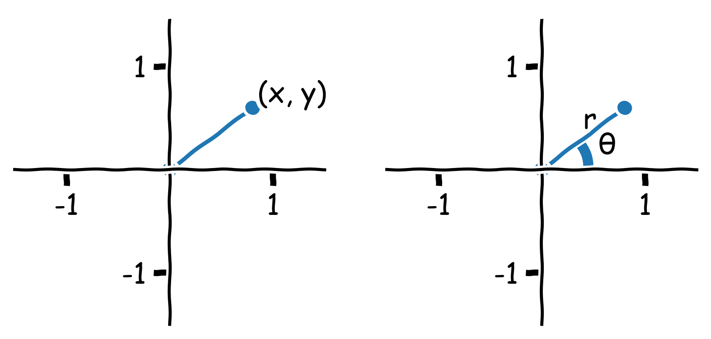
In the Vectors and Motion lesson, we introduced the idea of coordinates, which describe a point in space. In that lesson, we used something called ‘Cartesian coordinates.’ If we think of a line connecting the origin to a point, Cartesian coordinates provide the x and y position \((x, y)\). This is very useful for describing straight lines and many mathematical functions, such as those we created in the Intro to Animation adventure. In other cases, something called polar coordinates can be more useful. Polar coordinates define points in space differently. Rather than giving the x and y position, they specify points as their position on a circle. The two polar coordinates describes the radius of the circle (\(r\)) and its position around the circle, which is measured as the angle \(\theta\). Instead of reporting coordinates as \((x, y)\), polar coordinates are reported as \((r, \theta)\). This is easier to describe using a visual. In this image, we can see how the same point in space can be described using either Cartesian or polar coordinates.

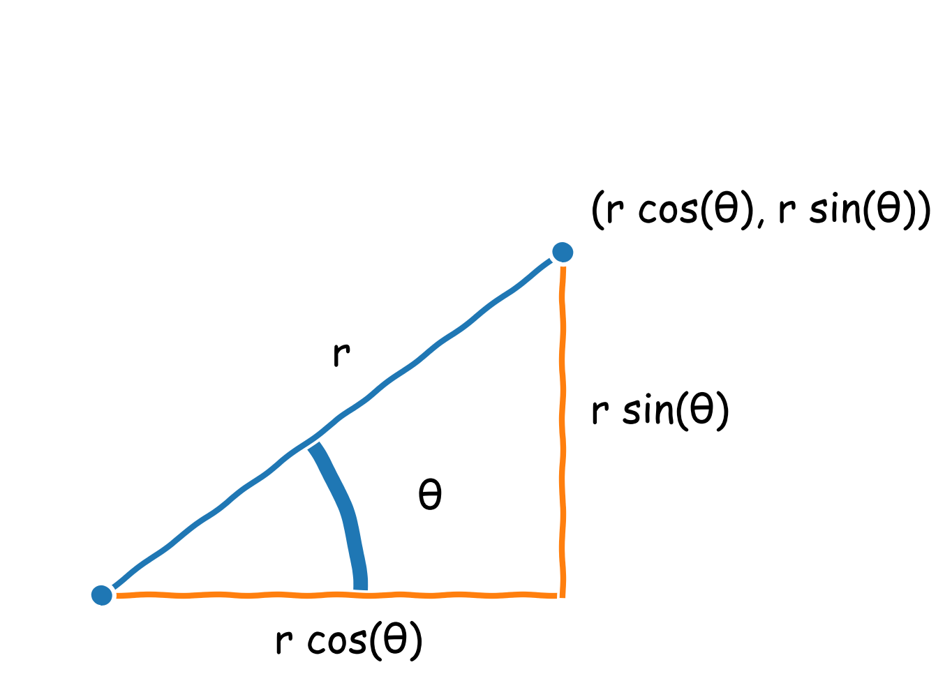
It sometimes is important to switch from Cartesian to polar coordiantes or in the reverse from polar to Cartesian coordinates. Luckily, there is an easy way to convert between these variables: \(x\) is simply the product of \(r\) and \(cos{\theta}\) : \[ x = r * \cos{\theta}\] \(y\), \(r\), and \(\theta\) are related to each other using the sin function where \[ y = r * \sin{\theta} \]

Going back to our discussion above about angular displacement, you can see how polar coordinates make it easy to describe the ball’s location. As the ball moves in a circle, we can describe its location using the radius and angle. This is much simpler than determining \(x\) and \(y\) for each position. Polar coordinates make it easier to describe the ball’s motion as well. By steadily increasing \(\theta\) (or the angle), you can draw a circle with a specific radius.

Summary

Let’s tie all of these concepts together to describe your ride on the merry-go-round! On your first ride, you chose a purple horse on the outer ring of the merry-go-round. Now, imagine a second ride where you chose the green horse that is closer to the senter instead. How would the following properties of your trip change: Angular displacement, angular velocity, linear velocity, angular acceleration?

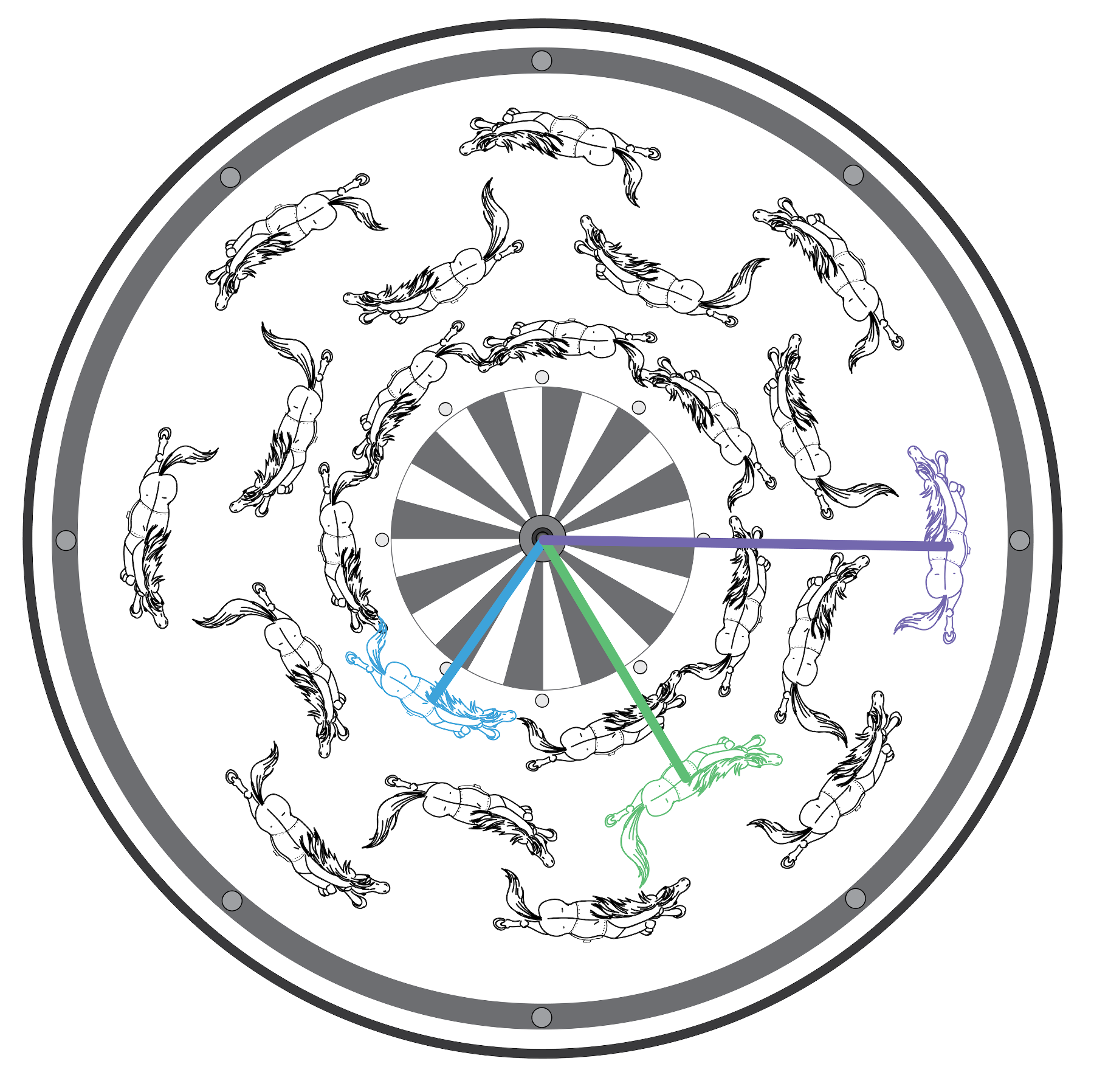
Your angular displacement, angular velocity, and angular acceleration would stay the same on both rides. In polar coordinates, the two horses have the same change in \(\theta\) coordinate but different but \(r\) values. Since \(\theta\) remains the same, both horses have equal angular displacements. For angular velocity and acceleration, every horse on the ride would have the same value. This is because the entire merry-go-round starts, moves, and stops together at the same rate.

What would change between the two horses is your linear velocity. Switching to a horse closer to the center (like the green horse) decreases \(r\) and means you are traveling in a smaller circle. Just like for the ball on a string, when \(r\) decreases, your linear velocity also decreases.

What about if your friend chose the horse in front of you? In this case, your initial \(\theta\) values would be different but your linear velocity and angular velocities would be identical for the entire ride. This is because you have the same \(r\) values and same change in \(\theta\) over time. What would be different if they chose the blue horse instead?

Finally, let’s think about how the ride changes over time? How would your angular acceleration change as you ride on the merry-go-round?

When you first get on the merry-go-round, your angular velocity and angular acceration are both zero. Once the merry-go-round starts moving, your angular velocity increases until it reaches a constant velocity. During that time, your angular acceleration will describe this increase in angular velocity. Eventually, the ride will reach a constant angular velocity that it will remain at for a most of the ride. At this point, your angular velocity is no longer changing and your angular acceleration is zero. At the end of the ride, your angular velocity is going to decrease back to zero at a rate controlled by the angular acceleration. Then once the merry-go-round has stopped moving, your angular velocity and acceleration are again zero.